Radiomics with Deep Learning | Mohammad Arafat Hussain, PhD

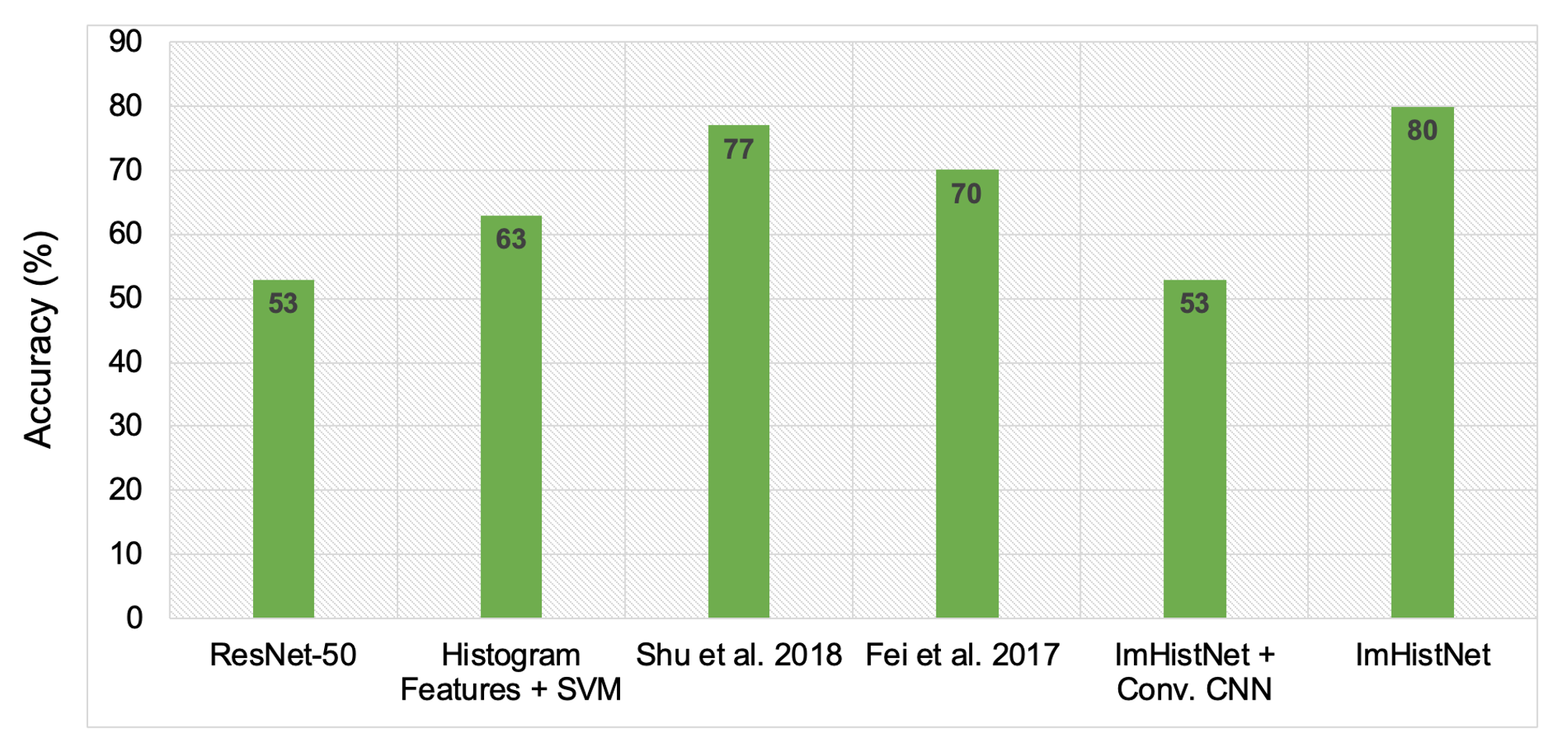
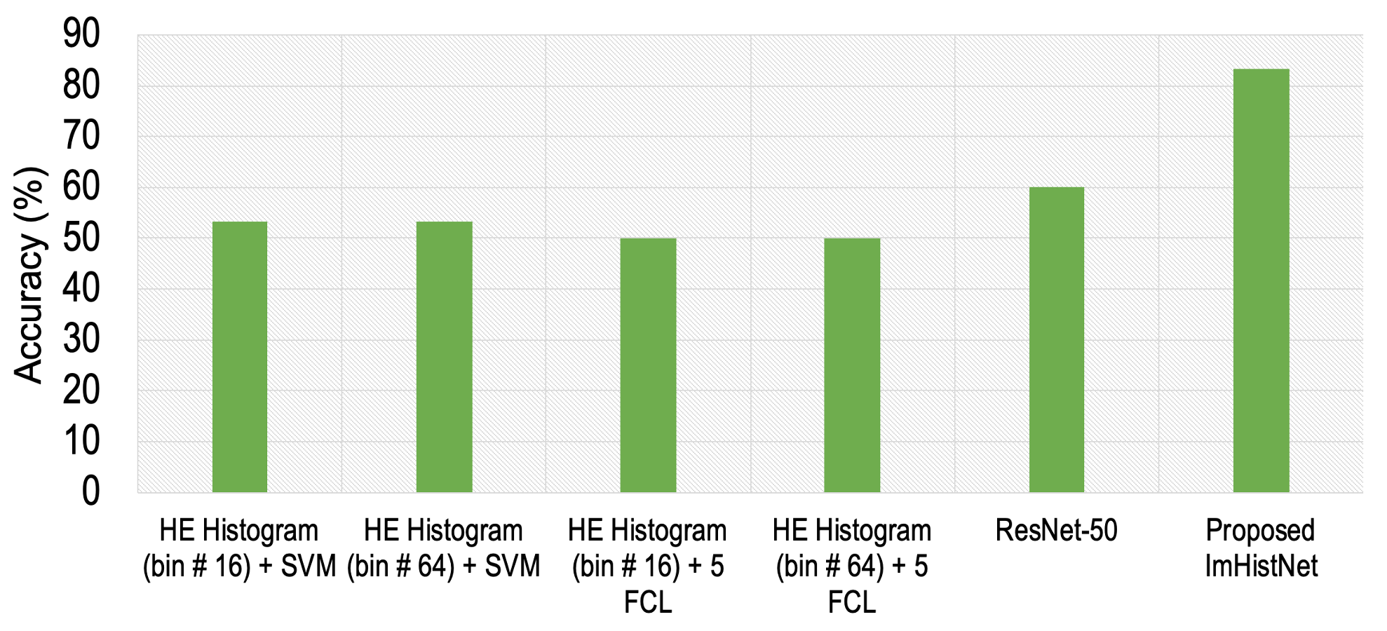
Fuhrman cancer grading and tumor-node-metastasis (TNM) cancer staging systems are typically used by clinicians in the treatment planning of renal cell carcinoma (RCC), a common cancer in men and women worldwide. Pathologists typically use percutaneous renal biopsy for RCC grading, while staging is performed by volumetric medical image analysis before renal surgery. Recent studies suggest that clinicians can effectively perform these classification tasks non-invasively by analysing image texture features of RCC from computed tomography (CT) data. However, image feature identification for RCC grading and staging often relies on laborious manual processes, which is error prone and time-intensive. To address this challenge, we developed a learnable image histogram in the deep neural network framework, named “ImHistNet”, that can learn task-specific image histograms with variable bin centers and widths. This approach enables learning statistical context features from raw medical data, which cannot be performed by a conventional convolutional neural network (CNN). The linear basis function of our learnable image histogram is piece-wise differentiable, enabling back-propagating errors to update the variable bin centers and widths during training. This novel approach can segregate the CT textures of an RCC in different intensity spectra, which enables efficient Fuhrman low (I/II) and high (III/IV) grading as well as RCC low (I/II) and high (III/IV) staging.

Learnable Image Histogram

Fig. 1: The graphical representation of the architecture of our learnable image histogram using CNN layers. We also break down our piece-wise linear basis function H_b^x on top of the figure in relation to different parts of the learnable image histogram architecture.

Our proposed learnable image histogram (LIH) stratifies the pixel values in an image x into different learnable and possibly overlapping intervals (bins of width w_b) with arbitrary learnable means (bin centers β_b). Given a 2D image (or a 2D region of interest or patch) x: R²→R, the feature value h_b^x: b ∈ B→R, corresponding to the number of pixels in x whose values fall within the b^th bin, is estimated as:

h_b^x = Φ{H^x_b} = Φ{max(0, 1−|x−β_b| × w_b)},

where B is the set of all bins, Φ is the global pooling operator, H_b^x is the piece-wise linear basis function that accumulates positive votes from the pixels in x that fall in the b>b^th</b> bin of interval [β_b-w_b/2, β_b+w_b/2], and w_b is the width of the b^th bin. Any pixel may vote for multiple bins with different H_b^x since there could be an overlap between adjacent bins in our learnable histogram. The final |B|×1 feature values from the learned image histogram are obtained using a global pooling Φ over each H_b^x separately.

ImHistNet Classifier Architecture

Fig. 2: Multiple instance decisions aggregated ImHistNet for RCC grade and stage classification. The light green block represents the proposed LIH layer shown in Fig. 1.

The classification network comprises ten layers: the LIH layer, five (F1-F5) fully connected layers (FCLs), one softmax layer, one average pooling (AP) layer, and two thresholding layers. The first seven layers contain trainable weights. The input is a 64×64 pixel image patch extracted from the kidney+RCC slices. During training, we fed randomly shuffled image patches individually to the network. The LIH layer learns the variables β_b and w_b to extract characteristic textural features from image patches. In implementing the proposed ImHistNet, we chose B = 128 and “average” pooling at H_b^x. We set subsequent FCL (F1-F5) size to 4096×1. The number of FCLs plays a vital role as the model’s overall depth is important for good performance. Empirically, we achieved good performance with five FCL layers. Layers 8, 9, and 10 of the ImHistNet are used during the testing phase and do not contain any trainable weights.

Data

We used CT scans of 159 patients from The Cancer Imaging Archive (TCIA) database. These patients’ diagnosis was clear cell RCC, of which 64 belonged to Fuhrman low (I/II), and 95 belonged to Fuhrman high (III/IV). Also, 99 patients were staged low (I-II), and 60 were staged high (III-IV) in the same cohort. The images in this database have variations in CT scanner models and spatial resolution. We divided the dataset for training/validation/testing as 44/5/15 and 75/5/15 for Fuhrman low and Fuhrman high, respectively. For anatomical staging, we divided the dataset for training/validation/testing as 81/3/15 and 42/3/15 for stage low and stage high, respectively. This database does not specify the time delay between the contrast media administration and acquisition of the image. Therefore, we cannot distinguish a CT volume in terms of the corticomedullary and nephrographic phase.

Results

Fig. 3: RCC grading performance by different methods, where the proposed method performed the best.

Fig. 4: RCC staging performance by different methods, where the proposed method performed the best.

For Details

Please read our papers [1], [2], [3]. Code can be found here.