Aggregated Orthogonal Decision CNN for Organ Localization

Automatic kidney localization in volumetric medical images is a critical step that often precedes subsequent data processing and analysis. For years, kidneys were typically localized manually in clinical settings. To automate this process, Criminisi et al. (2011, 2013) proposed regression-forest (RF)-based anatomy localization methods that predict the boundary wall locations of a tight region-of-interest (ROI) encompassing a particular organ. However, their reported boundary localization error for typical healthy kidneys (size ∼13×7.5×2.5 cm³) was 16 mm, which could significantly affect the subsequent volume estimation, depending on the volume estimation process. Cuingnet et al. 2012 fine tuned the method in (Criminisi et al. 2011) by using an additional RF, which improved the kidney localization accuracy by 60%. However, the authors mentioned (in Cuingnet et al. 2012) that their method was designed and validated with only non-pathological kidneys. Recently, Lu et al. 2016 proposed a right-kidney localization method using a cross-sectional fusion of convolutional neural networks (CNN) and fully convolutional networks (FCN) and reported a kidney centroid localization error of 8 mm. However, the robustness of this right-kidney-based deep learning model in localizing both kidneys is yet to be tested as the surrounding anatomy, and often locations, shapes and sizes of left and right kidneys are completely different and non-symmetric. As a priliminary work in this project, we proposed an effective deep CNN-based approach for tight kidney ROI localization, where orthogonal 2D slice-based probabilities of containing kidney cross-sections are aggregated into a voxel-based decision that ultimately predicts whether an interrogated voxel sits inside or outside of a kidney ROI.

Kidney Localization Using Orthogonal Decision Aggregated CNN

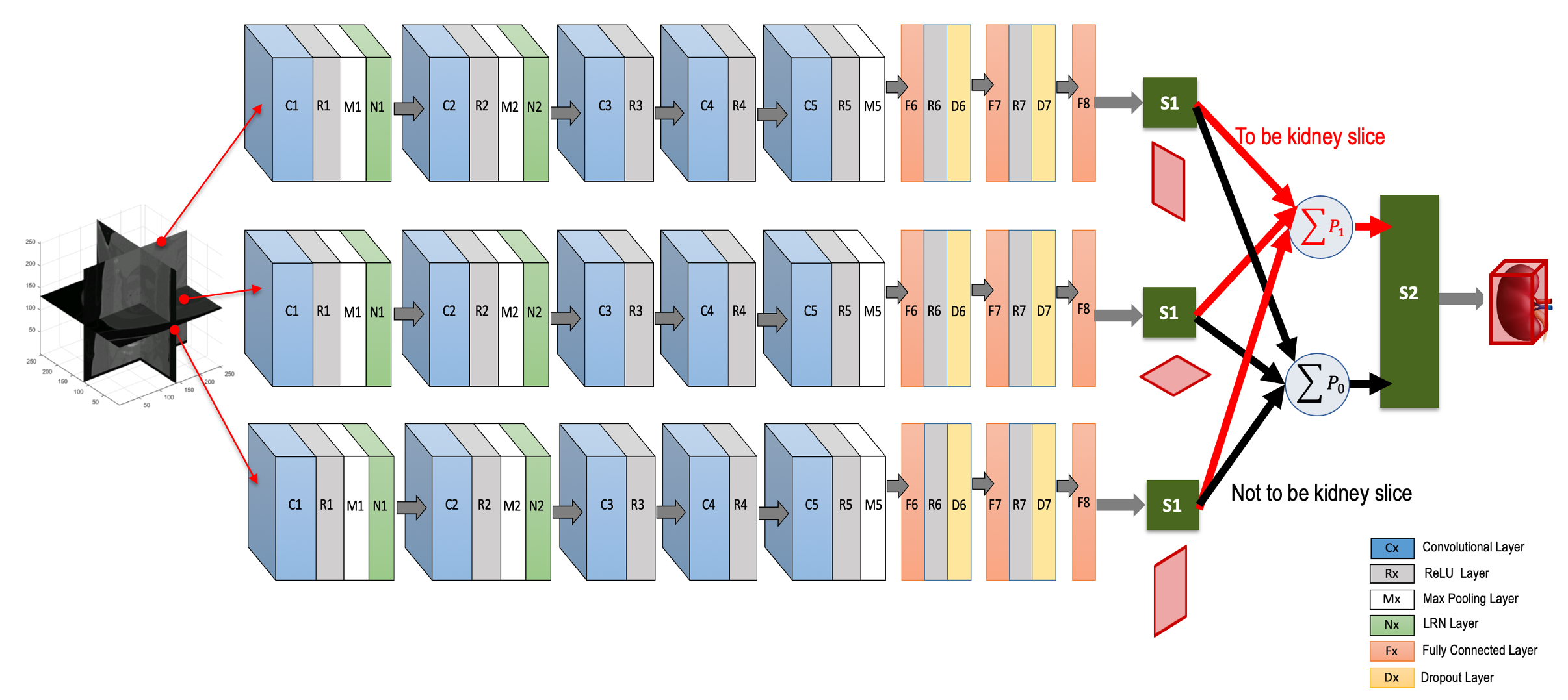
We use a deep CNN to predict the locations of six walls of the tight ROI boundary around a kidney by aggregating individual probabilities associated with three intersecting orthogonal (axial, coronal and sagittal) image slices (Fig. 1). The CNN has eleven layers excluding the input. It has five convolutional layers, three fully connected layers, two softmax layers and one additive layer. All but the last three layers contain trainable weights. The input is a 256×256 pixel image slice, either from the axial, coronal or sagittal directions, sampled from the initially generated local kidney-containing volumes. We train this single CNN (from layer 1 to layer 8) using a dataset containing a mix of equal numbers of 3D orthogonal image slices. Convolutional layers are typically used for sequentially learning the high-level non-linear spatial image features (e.g., object edges, intensity variations, orientations of objects etc.). Subsequent fully connected layers prepare these features for optimal classification of the object (e.g., kidney cross-section) present in the image. In our case, five convolutional layers followed by three fully connected layers make reasonable decision on orthogonal image slices if they include kidney cross-sections or not. During testing, three different orthogonal image slices are parallel-fed to this CNN and the probabilities for each slice of being a kidney slice or not are acquired at the softmax layer, S1 (Fig. 1). These individual probabilities from the three orthogonal image slices are added class-wise (i.e., containing kidney cross-section [class: 1] or not [class: 0]) in the additive layer, shown as P1 and P0 in Fig. 1. We then use a second softmax layer S2 with P1 and P0 as inputs. This layer decides whether the voxel where the three orthogonal input slices intersect is inside or outside the tight kidney ROI. The second softmax layer S2 is included to nullify any potential miss-classification by the first softmax layer S1. The voxels having probability (∈[0,1]) >0.5 at S2 are considered to be inside the kidney ROI. Finally, the locations of six boundary walls (two in each orthogonal direction) of this ROI are recorded from the maximum span of the distribution of these voxels (with probability >0.5) along three orthogonal directions.

Data

We used 100 patients’ CT scans accessed from the Vancouver General Hospital (VGH) records with required ethics approvals by the UBC Clinical Research Ethics Board (CREB), certificate number: H15-00237. There were a total of 200 kidney samples, and we used 130 samples (from 65 randomly chosen patients) for training, 20 samples (from 10 randomly chosen patients) for validation, and the remaining 50 samples for testing. Our dataset included 12 pathological kidney samples (with endo- and exophytic tumors), and our training and test data contained six pathological cases each. We made sure that kidneys from the same patient were not split across the training, validation, and test cases. These data were acquired using a Siemens SOMATOM Definition Flash (Siemens Healthcare GmbH, Erlangen, Germany) CT scanner. Ground truth kidney bounding boxes were calculated from manual kidney delineation performed by an expert radiologist.

Results

For Details

Please read our paper [1].