Deep Multiple Instance Learning for Cancer Detection

Renal cell carcinoma (RCC) is a common malignancy that accounts for a steadily increasing mortality rate worldwide. Widespread use of abdominal imaging in recent years, mainly CT and MRI, has significantly increased the detection rates of such cancers. However, detection still relies on a laborious manual process based on visual inspection of 2D image slices. In this work, we proposed an image collage based deep convolutional neural network (CNN) approach for automatic detection of pathological kidneys containing RCC. Our collage approach overcomes the absence of slice-wise training labels, enables slice-reshuffling based data augmentation, and offers favourable training time and performance compared to 3D CNNs. When validated on clinical CT datasets of 160 patients from the TCIA database, our method classified RCC cases vs. normal kidneys with 98% accuracy.

Why Multiple Instance Learning for RCC Detection?

Medical image analysis has enjoyed significant performance improvements through the use of various machine learning (ML) algorithms over the past few years. Most of these algorithms are fully supervised, requiring a large number of annotated datasets for model learning and prediction accuracy analysis. Unlike two dimensional (2D) single- or three-channel data (e.g., gray-scale or color images), which are most commonly used in computer vision tasks, three dimensional (3D) medical data presents different sets of challenges for ML approaches. For example, tissue abnormalities such as tumors, cancers, nodules, stones etc. are most often localized within a small region of anatomy and do not span the whole image volume. Localization and analysis of abnormal tissue are thus typically carried out on the 2D image slices. For example, staging of kidney tumors is done through slice-based tumor analysis and manual boundary tracing. However, image tags or labels (e.g. healthy, cancerous etc.) are mostly assigned per image volume or per patient basis. Therefore, all slices of an image are by default labeled with a single tag, though not all slices may contain the abnormal tissue. This scenario makes ‘single-instance’ ML approaches, especially deep learning ones such as convolutional neural networks (CNNs), very difficult to train on the 2D slices, as the input slice often does not correspond to the assigned volume-based label. A typical solution for this problem is to use the full 3D image volume as a single-instance for learning. However, 3D CNNs are considerably more difficult to train as they contain significantly more parameters and consequently require many more training samples, necessitate the use of expensive GPUs with very large memory, and require a lot more time to converge.

An alternative approach to single-instance learning is multiple-instance learning (MIL). MIL is a variation on weakly supervised learning wherein the learner receives a set of labeled bags, or ensembles, each containing multiple instances. This scenario allows the learner to label a bag with a class even if some or most of the instances within it are not members of that class. Using this MIL approach, the objective of our RCC detection application can be formulated such that a labelled bag corresponds to a labeled CT volume, and the constituting instances within the bag correspond to the CT’s 2D slices, some of which may contain RCC tumors while many may not. This reformulation allows us to correctly incorporate volume-based labels within an easy to train 2D slicebased CNN framework. In the context of deep learning on medical images, the joint benefits of MIL combined with the classification power of 2D CNNs have been recently demonstrated in a few applications including mammogram classification for breast cancer detection (Zhu et al. 2016), identifying anatomical body parts (Yan et al. 2016), colon cancer classification based on histopathology images (Xu et al. 2014), and classification of large 2D microscopy images (Kraus et al. 2016). To the best of our knowledge, such an approach has not been implemented specifically on 3D kidney data and a novel representation of volumetric CT data is necessary in order to extend such techniques for detection of RCC in CT data.

Collage Representation of 3D Image Data

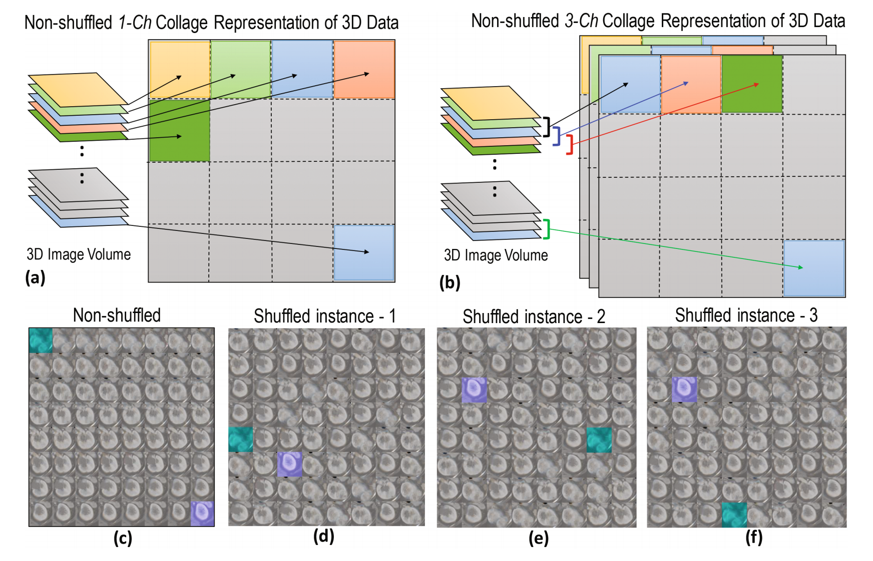
Typically, renal tumors grow in different regions of the kidney and are clinically scored on the basis of their CT slice-based image features such as size, margin (well-define or ill-defined), composition (solid or cystic), necrosis, growth pattern (endophytic or exophytic), calcification etc. Of course not all kidney slices necessarily contain tumors, nonetheless clinical labels (healthy/pathological) are normally recorded on a kidney- or a patient-basis. Therefore, it is not possible to use slice-based inputs in the training of a CNN because the volume-based label is not applicable to all constituent axial slices. To address this challenge, we propose a novel approach where the slices within the 3D image are rearranged into an extended 2D image collage (Fig. 1). In a non-shuffled collage representation, each consecutive image slice (for 1-channel) or, a group of n consecutive image slices (for n-channels, where n > 1) along a particular direction are sequentially placed on a 2D plane, which is schematically shown for a 1-channel and a 3-channels (n = 3) image in Fig. 1(a) and (b), respectively. Note that we opt to keep the collage dimension square (i.e. 512 × 512 pixel) in this experiment, however it is not a necessity. This collage not only ensures meaningful correspondence to the volume’s single label but also allows for invaluable data augmentation by simple random reshuffling of image slices as well as by rotation and flipping. A non-shuffled 2D image collage representing an actual kidney CT data and its shuffle-based three augmented collages are shown in Fig. 1(c) and (d)−(f), respectively. Note that we prepare our CNN input data in a process shown in Fig. 1(b), where we set n = 3. The resulting dimension of a single CNN input data is 512 × 512 × 3 pixel and the output was either 0 (healthy) or 1 (pathological).

Pathological vs Healthy Kidney Classification

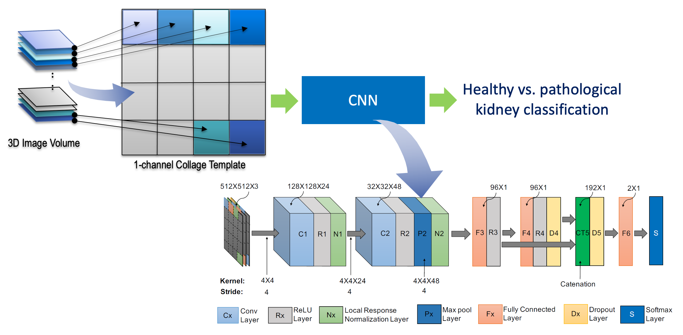
Our proposed CNN has seven layers excluding the input. All of these layers except the 5th layer (concatenation layer) contained trainable weights. Layer C1 is a convolutional layer that filters the input image with 24 kernels of size 4×4×3. Since we used collage-based image representation, we needed to carefully design our filter sizes and strides in a way that the convolutional (Cx) and max pooling (Px) filters do not overlap between two adjacent slices. To achieve this, we chose each edge size of the convolution filter to equal the stride in a particular layer. For example, the edge size of the convolution filter and the stride in the C1 layer were 4 and 4, respectively (Fig. 2). We chose a small convolutional filter size which tends to achieve better classification accuracy. Layer C2 is the second convolutional layer with forty eight 4×4×24 kernels applied to the output of C1. Unlike C1, we used a max pooling (P2) of 4×4×48 window in this layer to reduce the image size to 8×8 from 32×32. The output of C2 is connected to a fully connected layer (F3), which contains 96 units. Similarly, a layer F4 contains 96 units and is fully connected to F3. We concatenated the units of F3 and F4 into CT5 in order to reduce possible information loss. Note that the CT5 layer did not have any trainable weights. The CT5 layer is connected to an F5 layer having 2 units. These units are connected to a softmax layer (S), which produces the relative probabilities for back-propagation and classification.

Data

Our clinical dataset consisted of 160 kidney scans of 160 patients accessed from The Cancer Imaging Archive (TCIA) database. We used 80 healthy kidney samples from 80 patients who had one healthy kidney. The 80 pathological kidney samples used were from another 80 patient scans. Our dataset had variations in the scanner types, contrast administration, fields of view, spatial resolutions, and intensity (Hounsfield unit) ranges. The in-plane pixel size ranged from 0.58 to 1.50 mm and the slice thickness ranged from 1.5 to 5 mm. Of the 80 healthy and 80 carcinoma scans, we randomly chose 55 cases from each set to use for training and the remaining 25 for testing. Ground truth kidney RCC labels were also collected from the TCIA data records.

Results

For Details

Please read our [paper].